Category Archives: Electronics

Measuring the Speed of Sound

In the past on the "Don't Panic Geocast" we've talked about the speed of sound varying with temperature and how that can cause sound waves to bend. This phenomena, known as refraction, can result in all kinds of weird events, like being able to hear things from very far away when a thermal inversion is present in the atmosphere.

As I was researching some for that episode, I found that the standard formula for the speed of sound with temperature is a nice simple linear function over the ranges we care about. True, pressure and humidity can factor in there, but for simplicity, let's consider the largest factor... Temperature.

Formula for the speed of sound in dry air in m/s. Temperature is Celsius.

Formula for the speed of sound in dry air in m/s. Temperature is Celsius.

The formula above means that the speed of sound varies with temperature by 0.6 meters/second for every degree celsius of temperature change. That's about 2 ft/s for those of us more used to imperial units. A change that large should be pretty easy to see, right? This experiment and post were born from that statement.

To measure the speed of sound, I had several ideas. I could generate a short burst of noise and using an oscilloscope time how long it took to get to a microphone. That would require me to manually make the measurements, which probably means not a ton of data points since I'd have to either use the refrigerator to get a temperature difference or sit outside for a day. Neither of those were appealing. I ended up remembering some hardware that I had sitting around from the ultrasonic cave profiler.

The part of interest is the ultrasonic ranger. This little device (an SRF05) sends out a packet of ultrasonic pings and listens for their return. The device lets us know how long this takes by toggling an output from a digital 1 to digital 0. I already had the code to run this sensor, so I was half way there! The next thing I needed was a way to log the data. I didn't want to leave the door to the outside open to get power out there for the setup. I ended up using an SD card logger on top of the Arduino that was keeping track of the travel time.

Finally, we needed a target to range. Luckily, this was easy to do with some wood sticks, hot glue, and a plexiglass base plate. I glued the target to the base 260mm from where the pinger was mounted. After a couple of quick tests, I had verified that the setup was working! Adding a temperature and humidity sensor to the breadboard gave us everything we needed. Time to collect some data!
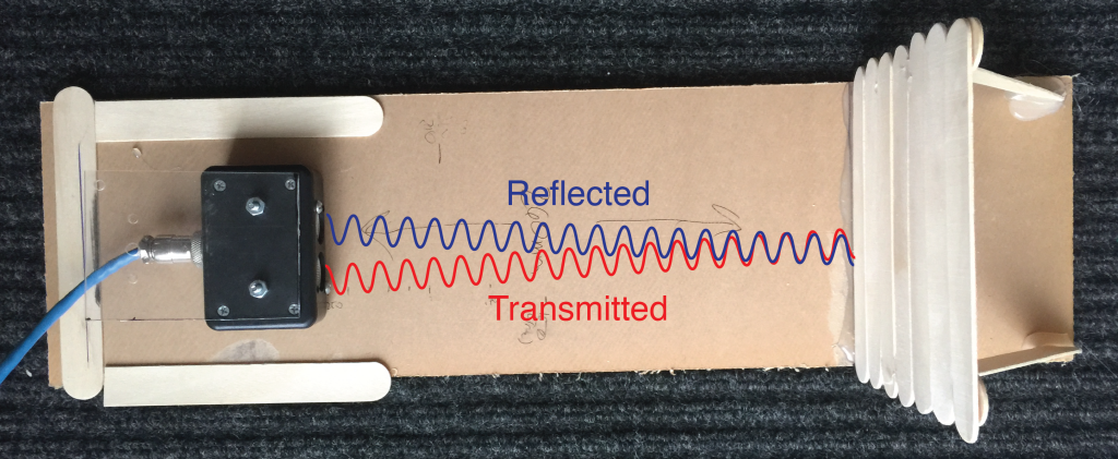
setup

Schematic of sound packets being transmitted and reflected. Really these are spherical wave-fronts, but the illustration is much cleaner this way!

Luckily, we've had pretty wide temperature swings during the day here in Pennsylvania lately. Using a decent sized 12V battery and voltage converter I could get days of run time on a single charge. To get the best data possible, I averaged many travel times per sample. This took less than a minute to do, which is fine since temperature isn't changing that rapidly.

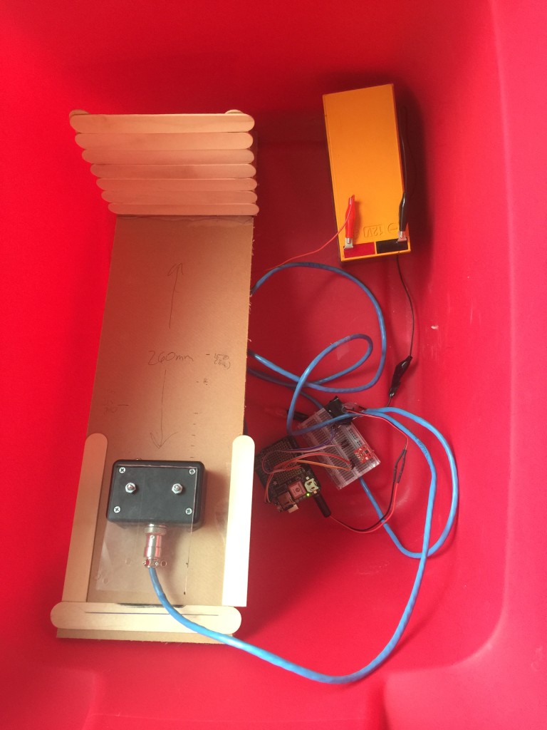
The complete setup in a tub ready to collect data outside.

The complete setup in a tub ready to collect data outside.

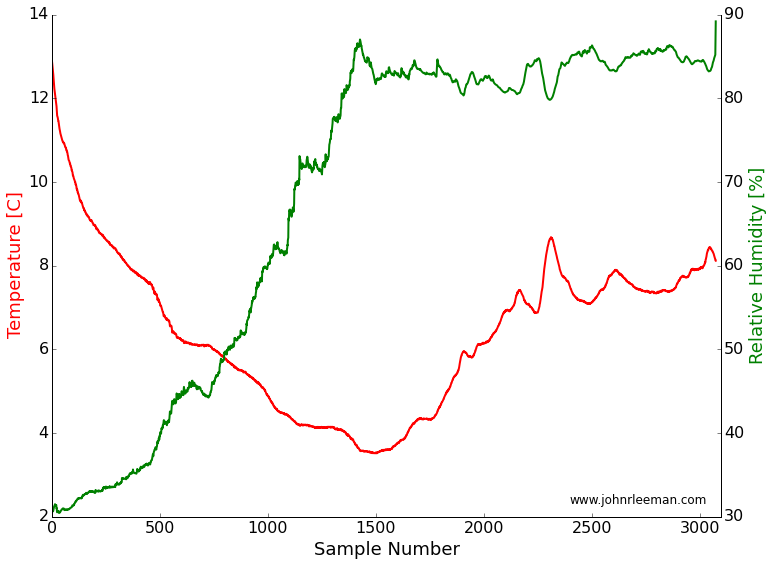
Now that a simple apparatus was complete, I placed it in a Rubbermaid tub to keep any stray precipitation (or the rodents) from damaging things. The data was stored in a text file containing two-way travel time to/from the target in microseconds, device estimated distance to target, and the temperature/humidity readings. I collected several days worth of data, each time slightly improving my recording setup to get the cleanest data. I had problems with days where the temperature varied very fast and it appears to have introduced noise, some days there was direct sunlight (a rare thing in the PA winters) that caused very high temperatures and convection in the tub. Finally, on the last day of my experiment, I got a nice data set. It was a day with slowly varying temperatures and mostly cloudy. I trimmed the ends of the data so things were equilibrated and got some decent results!

Temp_RH

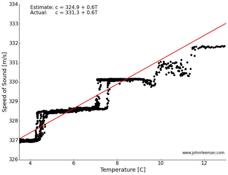
If we plot the temperature and the speed of sound against each other, we see what looks like a line! The steps are a result of being at the smallest increments in time that our system can sense. A better sensor could solve this, but for a rough estimate it turns out to be fine. Finding the best fit through this should tell us how well our measurements match the accepted formula. The slope of the line represents the rate of change of the speed with temperature (this should sound familiar to those calc. students out there), and the intercept represents the speed of sound at zero degrees.

Temp_Speed


We got the rate of change dead on! In fact we are within a few percent of the accepted value. The y-intercept is off by about 6 m/s, but I think that is a systematic offset due to a delay in the way the sensor is read. We could back that out, but maybe that is another topic for another time, or maybe we'll try this again with a different sensor. Please leave any comments or questions below!

Raindrops Keep Falling on my Radar - Part 2

Last time we looked at the raindrop fall speed of raindrops during a thunderstorm and compared the radar reflected power to my observations of the storm moving through State College. Today, thanks to Yvette Richardson and Bill Syrett from the Penn State Meteorology Department, we can compare the radar returns to actual weather station data. They were able to provide data from a weather station on top of the meteorology building on campus, about 3 miles from where my radar was located.

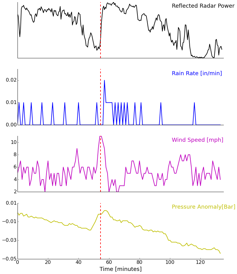
We expect more power to be returned to the radar during periods of heavy rain, so the main variable of interest is the rain rate. We'll plot up a couple of other meteorological variables just for fun as well. The weather station recorded observations every minute. I had to venture my best guess at the units based on their values. The rain rate values are low. Another station that I don't have the time-series for reported a maximum rain rate of 0.26 in/hr. Either way, let's examine the relative changes.

rain_wx_data_graph


Looking at the plot we can see that our prediction of higher rain rate equaling more reflected power holds. Unfortunately, the weather station didn't record precipitation rate with very fine resolution, so we really can only match the peak rain rate with the peak reflected power. The vertical red line marks the time of a weather service doppler radar screenshot we looked at in the last post that was right before the heaviest rain arrived. We also observe the higher wind speeds with the gust front ahead of the storm. As the storm passed over we saw decreasing pressures as well. The temperature and humidity aren't shown because they really weren't that interesting.

Now that we've verified our hypothesis (roughly anyway) about precipitation rate and radar return, we are ready to look at different types of reflectors. Next time, we will look at radar data collected during a snow storm for return intensity and the fall speed of snow flakes. That speed can be compared with video of falling snow for verification. Stay tuned!

Raindrops Keep Falling on my Radar - Part 1

What's the most complicated way to say it's raining? Well, if you know me, you know it will involve electronics, sensors, and signal processing! This post was originally going to compare the fall velocity for rain, sleet, and snow. Unfortunately, I haven't been lucky enough to be home to run my radar when it was snowing. It will happen this winter, but we'll start looking at some data now. Want to review radar before we get started? We have already talked about looking at the doppler signature of cars and got a tour of a mobile weather radar.

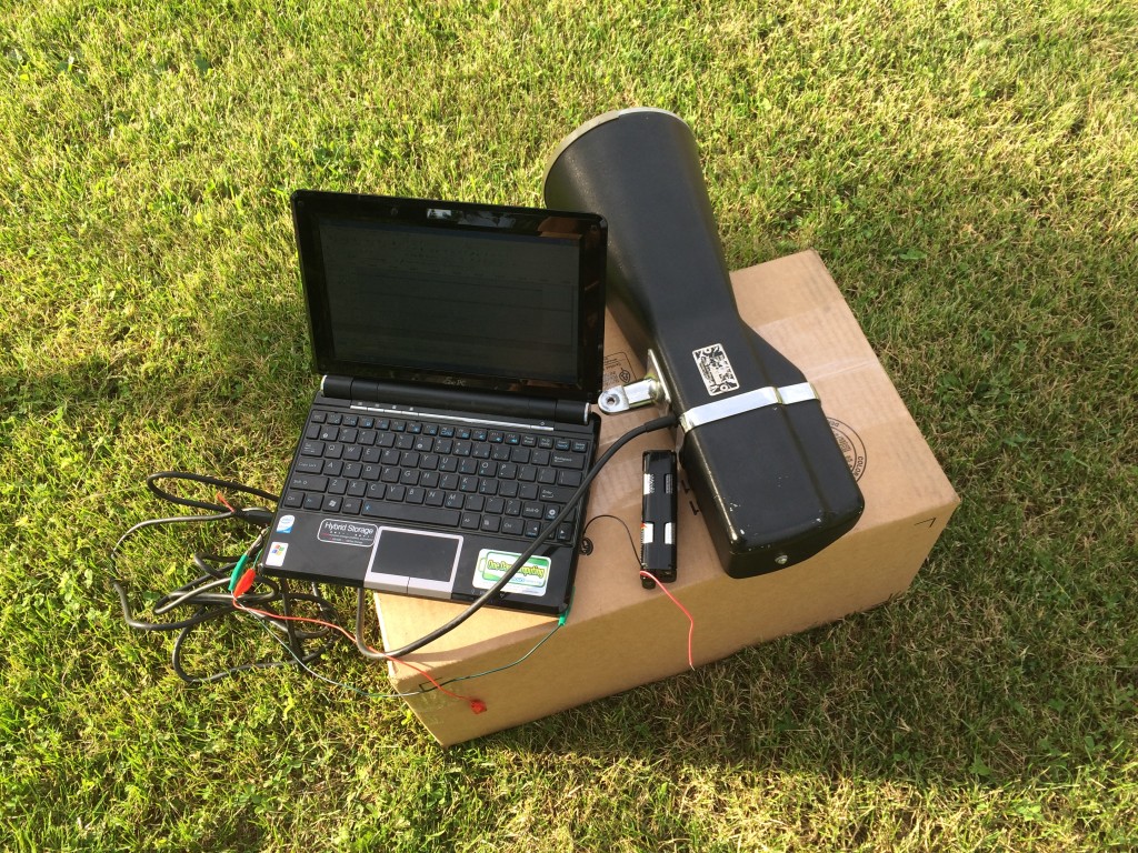
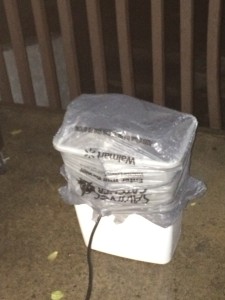
Back in October we had a couple of squall lines come through. On the 3rd, there was a significant event with two lines of storms. I had just been experimenting with measuring rainfall velocity with the modified X-band radar, so I decided to try another experiment. I put the radar unit in a trashcan and covered it with plastic bags. Then I sat it outside on our balcony and recorded for about 2.5 hours.

Testing the radar setup before the rain with some passing cars as targets.

Testing the radar setup before the rain with some passing cars as targets.

There is a radar in there! My make-shift rain proof radome. The only problem was a slight heat buildup after several hours of continuous operation.

There is a radar in there! My make-shift rain proof radome. The only problem was a slight heat buildup after several hours of continuous operation.

Not only do we get the doppler shift (i.e. velocity of the raindrops), but we get the reflected power. I'm not going to worry about calibrating this, but we can confidently say that the more (or larger) raindrops that are in the field of view of the radar, the more power will be reflected back.

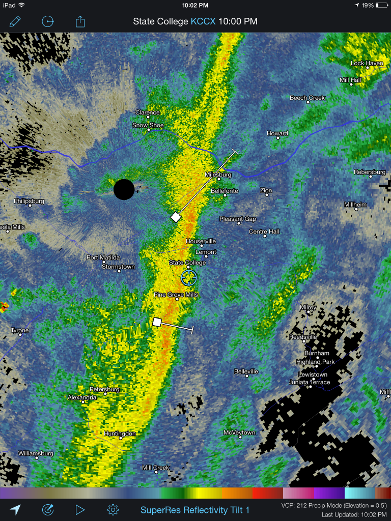
First, let's look at a screenshot of the local weather service radar. You can see my location (blue cross) right in front of the second line of showers. At this point we had already experienced one period of heavy rain and were about to experience another that would gradually taper off into a very light shower. This was one of the nicer systems that came through our area this fall.

A capture of our local weather radar, my location is the blue cross directly ahead of the storm.

A capture of our local weather radar, my location is the blue cross directly ahead of the storm.

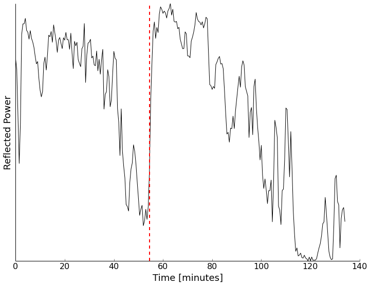
Now if we look at the returned power to the radar over time, we can extract some information. First off, I grouped the data into 30-second bins, so we calculate the average returned power twice per minute. Because of some 32-bit funny business in the computations, I just took the absolute value of the signal from the radar mixer, binned it, and averaged.

Reflected power received by the radar over time. The vertical red line is the time that the radar screen shot above was taken.

Reflected power received by the radar over time. The vertical red line is the time that the radar screen shot above was taken. We can see the arrival and tapering off of the storms.

From this chart we can clearly see the two lines of storms that came over my location. We also see lots of little variations in the reflected power. To me the rain-rate seemed pretty constant. My best guess is that we are looking at skewing of the data due to wind. This could be solved with a different type of radar, which I do plan to build, but that doesn't help this situation.

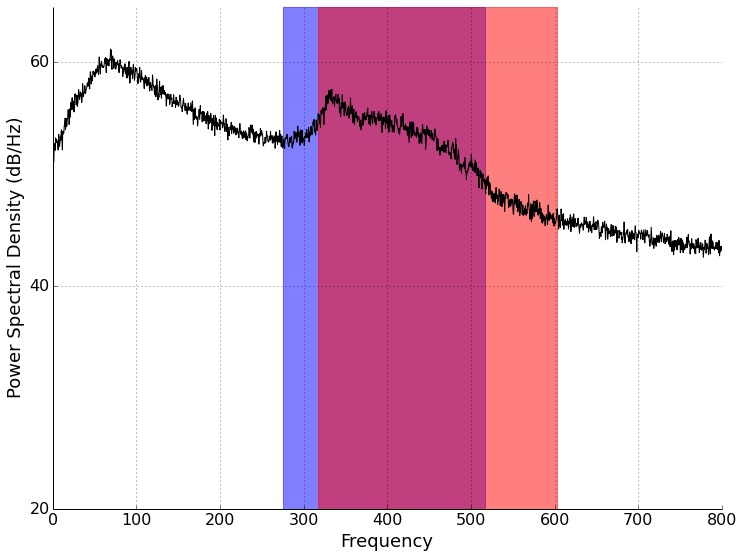
Let's look at what inspired this in the first place, the rainfall velocity. From a chart of terminal velocities, we can see that we expect to get drops falling between 4.03-7.57 m/s for moderate rain and 4.64-8.83 m/s for heavy rain. Taking a 5 minute chunk of data starting at 60 minutes into the data (during high reflectivity on the chart above), we can compute the doppler frequency content of the signal. Doing so results in the plot below, with the velocity ranges above shaded.

psd_velocity

Doppler frequency content of 5-minutes of data starting at 60 minutes into recording. The blue box shows doppler frequencies corresponding to moderate rain, and the red box corresponding to heavy rain.

Based on what I see above, I'd say that we fall right in line with the 0.25"-1" rain/hour data bracket! There is also the broad peak down at just under 100 Hz. This is pretty slow (about 1 m/s). What could it be? I'm not positive, but my best guess is rain splattering and rebounding off the top of my flat radar cap. I'm open to other suggestions though. Maybe part of this could be rain falling of the eve of the building in the edge of the radar view? The intensity seems rather high though. (It was also suggested that this could be a filter or instrument response artifact. Sounds like a clear air calibration may help.)

So, what's next? We'll take some clear-air calibration data and the use data from a Penn State weather station to see what the rain rate actually was and what the winds were doing. Maybe we can get a rain-rate calibration for this radar from our data. See you then!

Thank you to Chuck Ammon for discussions on these data!


Sensors, Sensors Everywhere!

This year at the fall meeting of the American Geophysical Union, I presented an education abstract in addition to my normal science content. In this talk, I wanted to raise the awareness of how easy it is to work with electronics and collect geoscience relevant data. This post is here to provide anyone that was at the talk, or anyone interested, with the content, links, and resources!

Sensors and microcontrollers and coming down in price thanks to mass production and advances in process technology. This means that it is now incredibly cheap to collect both education and research grade data. Combine this with the emergence of the "Internet of Things" (IoT), and it makes an ideal setup for educators and scientists. To demonstrate this, we setup a small three-axis magnetometer to measure the Earth's magnetic field and connected it to the internet through data.sparkfun.com. I really think that involving students in the data collection process is important. Not only do they realize that instruments aren't black boxes, that errors are real, and that data is messy, but they become attached to the data. When a student collects the data themselves, they are much more likely to explore and be involved with it than if the instructor hands them a "pre-built" data set.

For more information, watch the 5-minute talk (screencast below) and checkout the links is the resources section. As always, email, comments, etc are welcome and encouraged!

Resources

Talk Relevant Links

- Slides from the talk
- This blog! I post lots of electronics/data/science projects throughout the year.
- Raspberry Pi In The Sky
- Kicksat Project
- Weather Underground PWS Network
- uRADMonitor
- Our IoT magnetometer data stream
- Python Notebooks
- GitHub repository for the 3D Compass demo
- AGU Pop-Up Session Blog

Parts Suppliers

- Adafruit
- Sparkfun
- Digikey
- Element14

Assorted Microcontrollers/Computers

- Beagle Bone
- Raspberry Pi
- Arduino
- Propeller
- MBed
- Edison
- MSP430
- Light Blue Bean

General

- Thingiverse 3D printing repository
- Maker blogs from places like Hackaday, MAKE, Adafruit, Sparkfun, etc

Doppler On Wheels - A Tour of a Mobile Radar

DOW7_Web

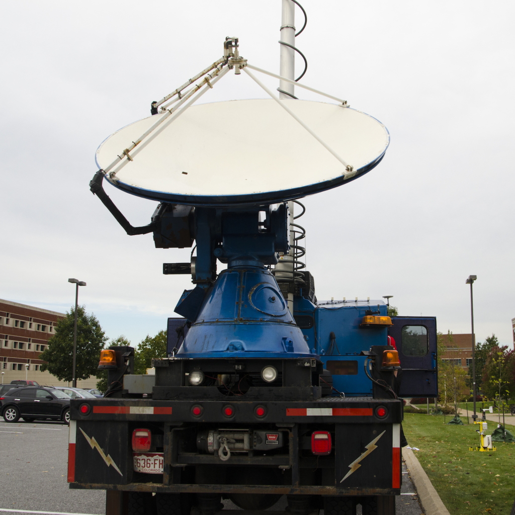
Recently, Penn State was lucky enough to have the "Doppler on Wheels" or DOW visit for two weeks through an NSF education grant! The truck, owned and operated by the Center for Severe Weather Research, is probably familiar to you if you have watched any of the storm chasing television shows or are interested in severe storms.  Dr. Yvette Richardson and Dr. Matt Kumjian were the faculty hosts and incorporated the radar into classes they are teaching.

I've always believed in getting students involved with data collection.  If students collect the data, they are attached to it and begin to see the entire scientific process.  Data doesn't just appear, real data is collected, often with complex instruments, and processed to remove various problems, corrections, etc.  It's not everyday that students get to collect data with a state-of-the-art radar though!

For this entry we're going to try a video format again.  Everyone seemed to like the last video entry (Are Rocks like Springs?).  Keep the feedback coming! It was a bit windy, but I've done what I can with the audio processing.  A big thanks to everyone who let me talk with them!  As always, keep updated on what's happening by following me on twitter (@geo_leeman).  This week I'll be off to New York to hear Edward Tufte talk about data visualization, so expect updates about that!

Mythbusting: Cooling a Drink with a Wet Paper Towel

While reading one of the many pages claiming to have "15 Amazing Life Hacks" or something similar, I found a claim about quickly cooling a drink that deserved some investigation.  The post claimed that to quickly cool your favorite drink you should wrap the bottle/can in a wet paper towel and put it in the freezer.  Supposedly this would quickly cool the drink, faster than just the freezer.  My guess is that the thought process says evaporative cooling is the culprit.  This is why we sweat, evaporating water does indeed cool the surface.  Would water evaporate into the cold, but dry freezer air? Below we'll look at a couple of experiments and decide if this idea works!

We will attack this problem with two approaches.  First I'll use two identical pint glasses filled with water and some temperature sensors, then we'll actually put glass bottles in and measure just the end result.  While the myth concerns bottles, I want to be able to monitor the temperature during the cooling cycle without opening the bottles.  For that we'll use the pint glasses.  

First I had to build the temperature sensors.  The sensors are thermistors from DigiKey since they are cheap and relatively accurate as well.  To make them fluid safe, I attached some three-lead wire and encapsulated the connections with hot-glue.  The entire assembly was then sealed up with heat-shrink tubing.  I modified code from an Adafruit tutorial on thermistors and calibrated the setup.  

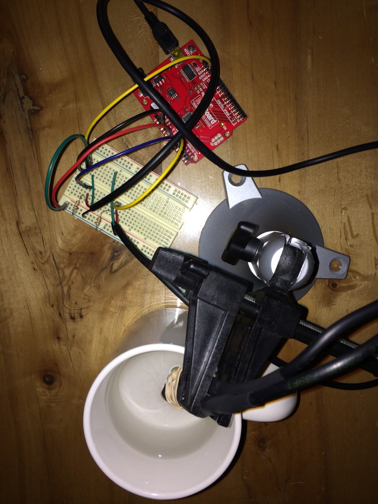
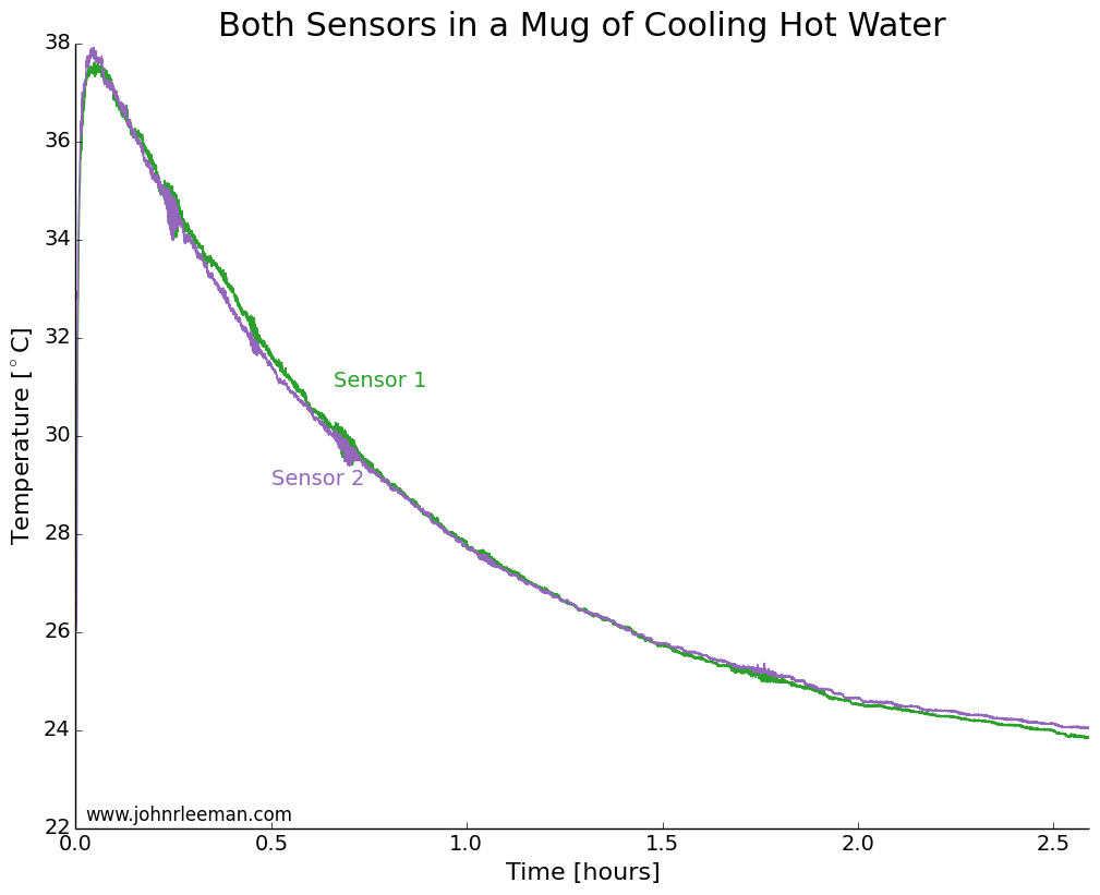
To make sure that both sensors had a similar response time, we need to do a simple control test.  I placed both probes in a mug of hot water right beside each other.  We would expect to see the same cooling at points so close together, so any offset between the two should be constant.  We also expect the cooling to follow a logarithmic pattern.  This is because the rate of heat transfer is proportion to the temperature difference between the water and the environment (totally ignoring the mug and any radiative/convective transfer).  So when the water is much hotter than the air, it will cool quickly, but when it's only slightly hotter than the air it will take much longer to cool the same amount.  

Mug Cooling Photo

Plotting the data, we see exactly the expected result.  Both sensors quickly rise to the water temperature, then the water cools over a couple of hours.  The noisy segments of data about 0.25 hrs, 0.75 hrs, and 1.75 hrs in are likely interference from the building air conditioning system.  

CoolingWater_AbsoluteTemps

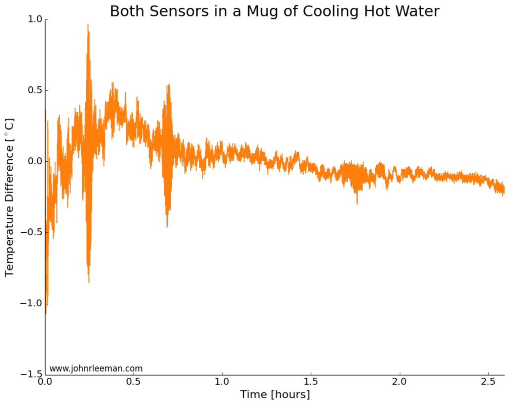
If we plot the temperature difference between the sensors it should be constant since they are sensing the same thing.  These probes look to be about dead on after calibration.  Other than the noisy segment of data, they are always within 0.5 degrees of each other.  Now we can move on to the freezer test.

CoolingWater_TempDifference

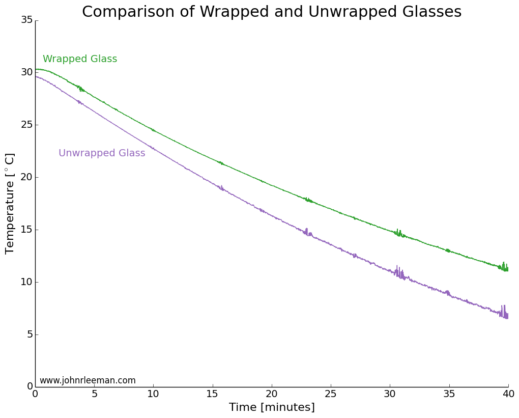
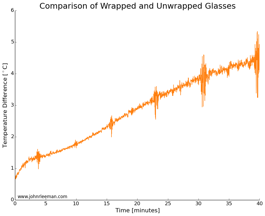
I used two identical pint glasses and made thermocouple supports with cardboard.  One glass was wrapped in tap water damped paper towel, the other left as a control.  Both were inserted into the freezer at the same time and the temperature monitored.  The water was initially the same temperature, but the readings quickly diverged.  The noisy data segments reappear at fixed intervals suggesting that the freezer was turning on and off.  The temperature difference between the sensors grew very quickly, meaning that the wrapped glass was cooling more slowly than the unwrapped glass.  This is the opposite of the myth! 

FreezingWater_AbsoluteTemps


FreezingWater_TempDifference

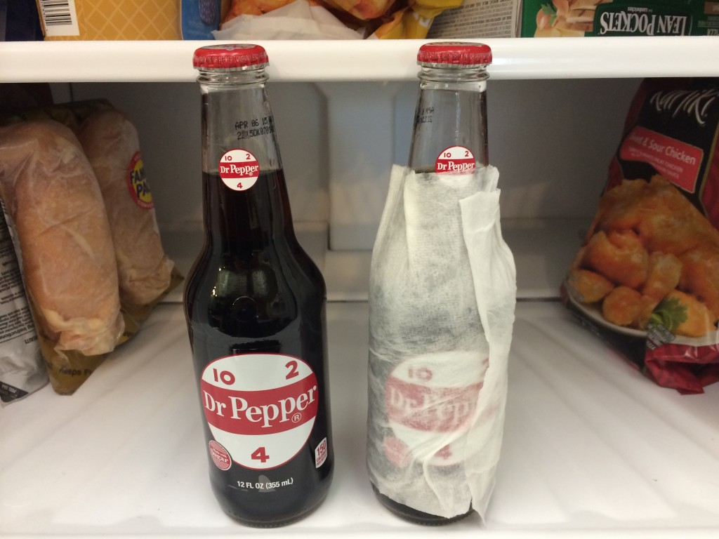
Next I placed two identical, room temperature bottles of soda in the freezer, again with one wrapped and one as a control.  After 30 minutes in the freezer, the results showed that the bottles and their contents were practically identical in temperature.  The wrapped bottle was slightly warmer, but it was within the resolution of the instruments (thermocouple and IR sensor).  I did this test multiple times and always got temperatures within 1 degree of each other, but not consistently favoring one bottle.

So what's happening here? Well, I think that the damp paper towel is actually acting as a jacket for the beverage.  Much like covering yourself when it's cold outside, the damp paper towel must be cooled, then the beverage can cool.  Adding that extra thermal mass and extra layer for the heat to diffuse through.  To provide another test of that hypothesis I again tested bottles with a control and a foam drink cooler around the base.  The foam cooler did indeed slow the cooling, the bottle being several degrees warmer than the control.

2014-08-13 17.56.28

The last question is why did the test with the glasses show such a pronounced difference, but the bottle test show no difference? My best guess is that the pint glass was totally wrapped vertically and that bottle had the neck exposed still.  Another difference could be the thickness of the towel layer and the water content of the towels.  

The Conclusion: BUSTED! Depending on how you wrap the paper towel it will either have no effect or slow down the cooling of your favorite drink.  

Let me know any other myths I should test! You can also keep up to date with projects and future posts by following me on twitter (@geo_leeman).

Arduino Code:

// which analog pin to connect
#define THERMISTOR1PIN A0
#define THERMISTOR2PIN A1
// resistance at 25 degrees C
#define THERMISTORNOMINAL 10000
// temp. for nominal resistance (almost always 25 C)
#define TEMPERATURENOMINAL 25
// how many samples to take and average, more takes longer
// but is more 'smooth'
#define NUMSAMPLES 15
// The beta coefficient of the thermistor (usually 3000-4000)
#define BCOEFFICIENT 3950
// the value of the 'other' resistor
#define SERIESRESISTOR1 9760
#define SERIESRESISTOR2 9790

int samples1[NUMSAMPLES];
int samples2[NUMSAMPLES];

void setup(void) {
Serial.begin(9600);
analogReference(EXTERNAL);
}

void loop(void) {
uint8_t i;
float average1;
float average2;

// take N samples in a row, with a slight delay
for (i=0; i< NUMSAMPLES; i++) {
samples1[i] = analogRead(THERMISTOR1PIN);
samples2[i] = analogRead(THERMISTOR2PIN);
delay(10);
}

// average all the samples out
average1 = 0;
average2 = 0;
for (i=0; i< NUMSAMPLES; i++) {
average1 += samples1[i];
average2 += samples2[i];
}
average1 /= NUMSAMPLES;
average2 /= NUMSAMPLES;

//Serial.print("Average analog reading ");
//Serial.println(average);

// convert the value to resistance
average1 = 1023 / average1 - 1;
average1 = SERIESRESISTOR1 / average1;

average2 = 1023 / average2 - 1;
average2 = SERIESRESISTOR2 / average2;
//Serial.print("Thermistor resistance ");
Serial.print(average1);
Serial.print(',');
Serial.print(average2);
Serial.print(',');

float steinhart;
steinhart = average1 / THERMISTORNOMINAL; // (R/Ro)
steinhart = log(steinhart); // ln(R/Ro)
steinhart /= BCOEFFICIENT; // 1/B * ln(R/Ro)
steinhart += 1.0 / (TEMPERATURENOMINAL + 273.15); // + (1/To)
steinhart = 1.0 / steinhart; // Invert
steinhart -= 273.15; // convert to C

Serial.print(steinhart);
Serial.print(',');

steinhart = average2 / THERMISTORNOMINAL; // (R/Ro)
steinhart = log(steinhart); // ln(R/Ro)
steinhart /= BCOEFFICIENT; // 1/B * ln(R/Ro)
steinhart += 1.0 / (TEMPERATURENOMINAL + 273.15); // + (1/To)
steinhart = 1.0 / steinhart; // Invert
steinhart -= 273.15; // convert to C(steinhart);

Serial.println(steinhart);
//Serial.println(" *C");

delay(1000);
}

Are Rocks like Springs? A Video Demonstration

Today I was getting a demo in the lab ready for a tour group and decided to try shooting a quick, unscripted bit on rocks as springs.  There are a few generalized statements in here, but overall it is a first try at a public education video.  Comments welcome!

Doppler Radar at Home: Experiments with a CW Radar Part 1

When you hear "radar", you probably think of weather radar and a policeman writing a ticket.  In reality there are many kinds of radar used for everything from detecting when to open automatic doors at shops to imaging cracks in concrete foundations.  I've always found radar and radar data fascinating.  Some time back I saw Dr. Gregory Charvat modify an old police radar on YouTube and look at the resulting signal.  I happened to see that model of radar (a 1970's Kustom Electronics) go by on EBay and managed to buy it.  I'm going to present several experiments with the radar over a few posts.  If you want to learn more about radar and the different types of radar I highly recommend Dr. Charvat's book Small and Short-Range Radar Systems.  I haven't bought a personal copy yet, but did manage to read a few chapters of a borrowed copy.

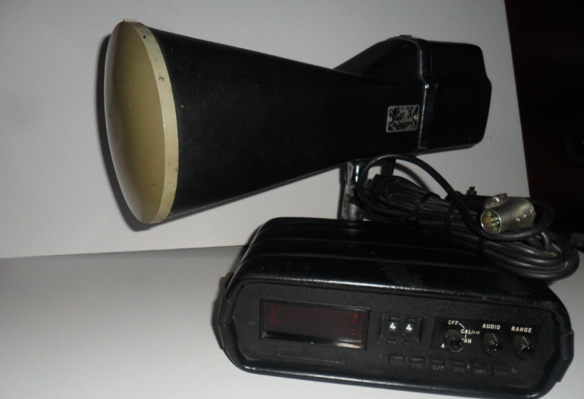
The doppler radar I purchased.  I'm not using the head unit.

The doppler radar I purchased. I'm not using the head unit.

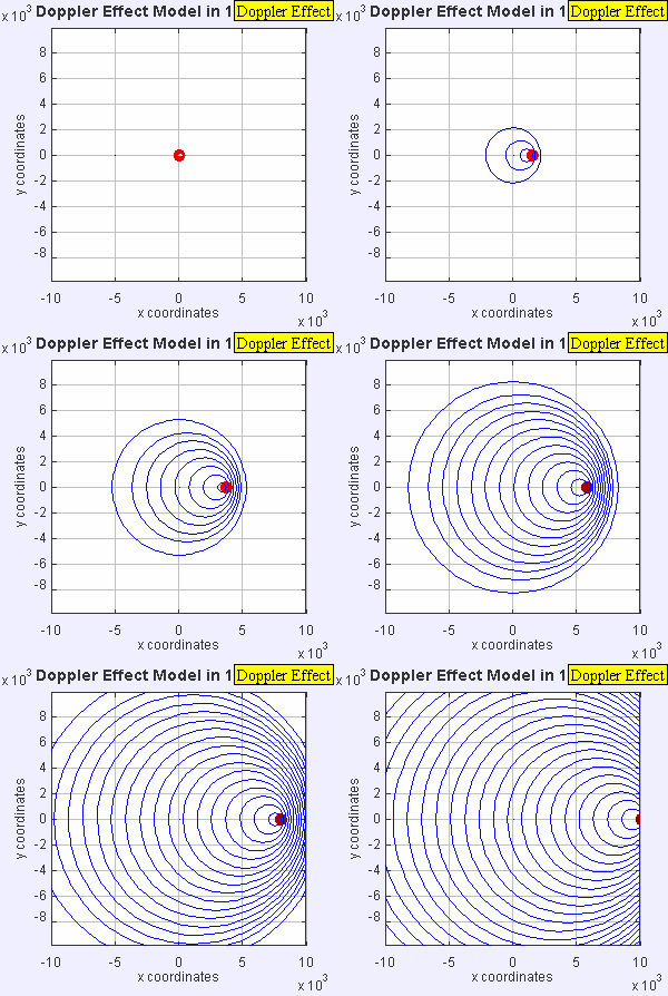
The radar I have outputs the doppler shift of a signal that is transmitted, reflected, and received.  Doppler is familiar to all of us as we hear the tone of a train horn or ambulance change as it rushes past us.  Since there is relative motion of the transmitter (horn) and receiver (your ears), there is a shift in received frequency.  Let's say that the source emits sound at a constant number of cycles per second (frequency).  Now let's suppose that the distance between you and the source begins to close quickly as you move towards each other.  The apparent frequency will go up because the source is closer to you each emitted cycle and you are closer to the source!

The doppler effect of a moving source.  Image: Wikipedia

The doppler effect of a moving source. Image: Wikipedia

This particular radar transmits a signal at a frequency of 10.25 GHz.  This outgoing signal is continually transmitted and reflected/scattered off of objects in the environment.  If the object isn't moving, the signal returns to the radar at 10.25 GHz.  If the object is moving, the signal experiences a doppler shift and the returned frequency is higher or lower than 10.25 GHz (depending on the direction of travel).  This particular radar can be easily hacked and we can record the doppler frequency out of a device called a mixer.  The way this unit is designed, we can't tell if the frequency went up or down, just how much it changed.  This means we don't know if the targets (cars) are coming or going, just how fast they are traveling.  Maybe in a future set of posts, we'll build a more complex radar system such as the MIT Cantenna Radar.  Be sure to comment if that's something you are interested in.

Since we'll be measuring speeds that are "slow" compared to the speed of light, we can ignore relativistic effects and calculate the speed of the object knowing the frequency change from the mixer, and the frequency of the radar.

Simplified doppler velocity.

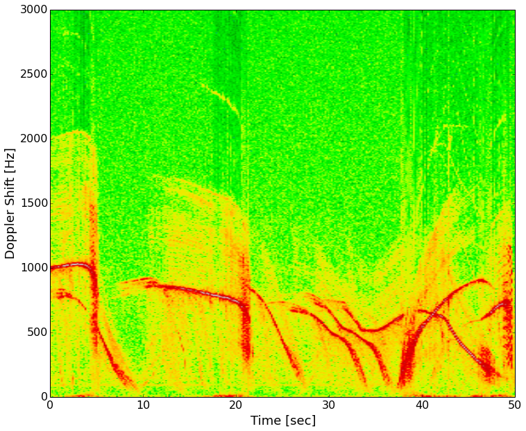
I took the radar out to the street and recorded several minutes of traffic going by, including city busses.  Making a plot of the data with time increasing as you travel left to right and doppler frequency (speed) increasing bottom to top, we get what's known as a spectrogram.  Color represents the intensity of the signal at a given frequency at a certain point in time.

Speeds of several cars on my street.  1000 Hz is about 33 mph and 500 Hz is about 16 mph.

Speeds of several cars on my street. 1000 Hz is about 33 mph and 500 Hz is about 16 mph.

The red lines are strong reflectors (the cars).  Most of the vehicles slow down and turn on a side street in front of the radar.  About 30 seconds in there are three vehicles, two slow down and turn, the third again accelerates on past.  Next I'll be lining up a video of these cars passing the radar with the data and you'll be able to hear the doppler signal.  To do that I'm learning how to use a video processing package (OpenCV) with Python.

In the next few installments, we'll look at videos synced with these data, radar signatures of people running, how radar works when used from a moving car, and any other good targets that you suggest!

Reviving a Piece of the 1970's: ISEE-3

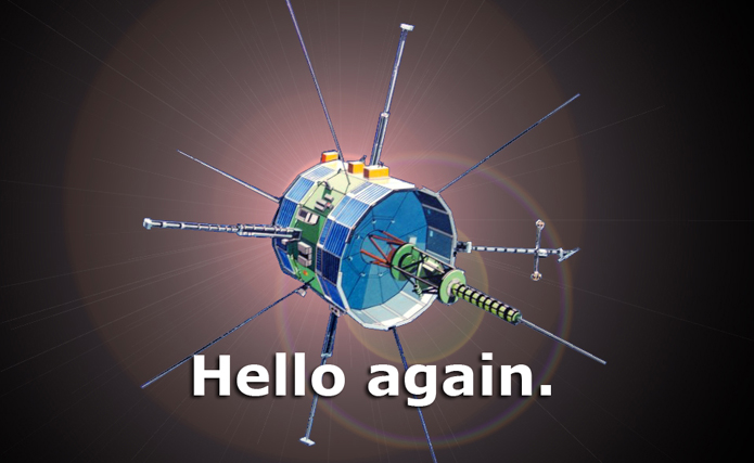
hello.again.m

There's been a decent buzz in the space and tech communities about the "ISEE-3 Reboot Project", so I thought it would be worth mentioning here and pointing out some of wonderful techniques they are using to revive a satellite from almost 40 years ago.

The ISEE-3 satellite is one of three satellites that made up the International Cometary Explorer (ICE) program.  There were some interesting orbital things done with this satellite after its launch in August of 1978.  It was also the first spacecraft to go through the tail of a comet!  As with all missions, this one came to an end and the satellite was not head from since 1998.  The equipment to talk to the satellite was removed and it was considered to be out of service.

ISEE-3 sits in a heliocentric orbit, meaning that orbits the sun, not the Earth.  We knew that ISEE-3 would make another stop by our planet in 2014 when it was parked in this orbit in 1986 (from what I can tell anyway).  A group of citizen scientists started the ISEE-3 Reboot project, crowd funded on the internet.  They got permission to take over the satellite and intend to use the Moon's gravity and a rocket burn to send it on another mission.  If the window of June is missed, the satellite will probably never be heard from again.

The team was able to contact ISEE-3 on May 29 using the Arecibo observatory radio telescope.   The craft was commanded to transmit engineering telemetry, basically a health screening of the systems.  The team is currently busy decoding the data (streaming in at 512 bits/sec) and planning how they will execute the rocket burn.

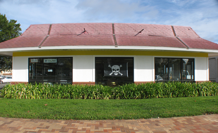
The team is running out of an old McDonalds at the NASA Ames Research Park, the makeshift mission control has been termed "McMoons" after hosting previous space based projects.

IMG_3113


The part of this that I find amazing is the role that software defined radio is playing.  Software defined radio (SDR) is a way to use software to emulate radio equipment.  With a small USB stick I can receive many different kinds of radio signals and decode them, something that would have required racks of equipment a few years ago.  This team is using a radio termed the "USRP" that allows them to transmit and receive.  I've written about them before (here) and have used them in research.  They are amazing little units and provide a unique learning opportunity.  (Maybe I'll post something about a radar we made with one of them as a demo!)  A photo tweeted by the team shows 2 USRP units and laptops hooked into the giant dish antenna at Arecibo.

Screen Shot 2014-06-02 at 12.51.08 PM


That's all for now, but stay tuned to the team's website for updates and I'll be keeping up with the progress as well.  This is just another incredible example of how advanced hardware and software that has become relatively cheap can allow a group of savvy citizens to accomplish incredible feats!  Way to go folks!


Drawdio: Creating Music with Your Hands

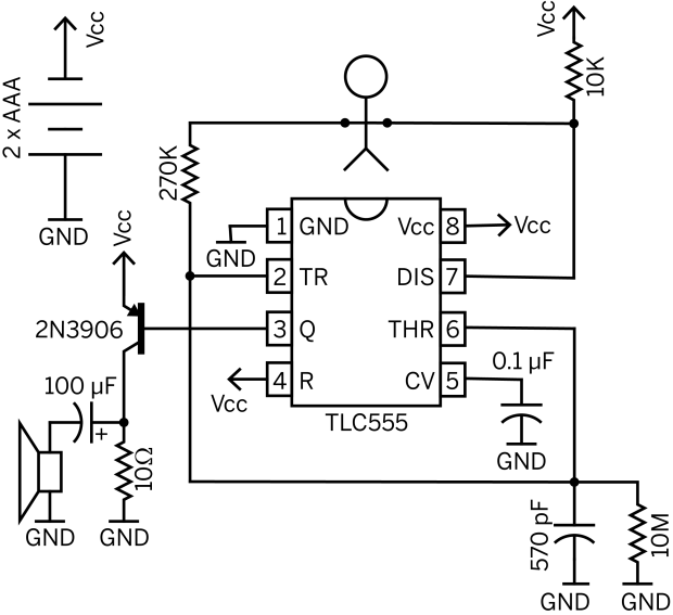
Awhile back I saw a post from the folks at the MIT Media Lab on a little creation they called the "drawdio" (here).  This looked like a fun little project! It's an oscillator based on the classic 555 timer integrated circuit, but with a twist.  The twist is that you can control the frequency of the oscillation (tone of the note played by a speaker) by varying the resistance between two contacts.  These contacts seem to commonly be a pencil lead and your body, but as the MIT website demonstrates, almost anything can be used.

Schematic: Make.com

Schematic: Make.com

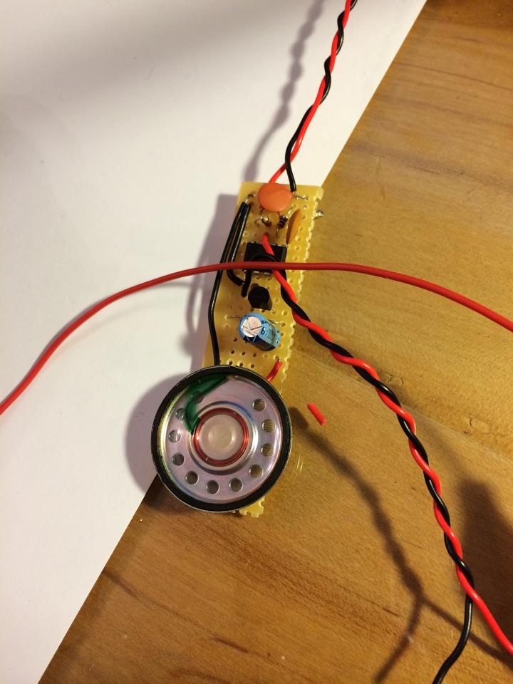
I decided it was time to build one of these, so I headed over the MAKE to get the plans.  I already had most of the parts (or good substitutes) on hand.  The battery holder and enclosure would have to come later.  I built the circuit with simple point-to-point wiring on perforated board.  The speaker is a salvaged part from a fax machine!

Drawdio No Case


I plugged the power supply in a touched the signal wires together.  The speaker let out a shrill tone and we were in business.  The next challenge was figuring out a case a final setup for the device.  I wanted this to be durable since lots of people at work and home would be playing with it.  The solution ended up being hot glue and a plastic crayon case.  I drilled holes in the case above the speaker for sound and added a power switch.  The final touch was terminal posts for the sense wires that control the pitch.

To make the sensor I just wrapped bare wire around a pencil body for one contact and inserted a push pin into the lead at the top for a second contact.  The goal is to complete that circuit and change the resistance between the two contacts.  The easiest way is to draw a graphite track on paper and make the circuit through your hands.  See the demo video below.

This is an incredibly fun project and can be very educational to the beginning electronics hobbyist or a way to get school children interested in STEM fields.  What are you waiting for? Go build a drawdio! (Kits available from Adafruit)